I found that picking the right activation function for a Bayesian Neural Network lets you compute uncertainty analytically in a single forward pass instead of running 50 Monte Carlo samples. 18x faster inference. The math works because Gaussian-family distributions have closed-form moments under exponential-quadratic activations, a property that goes back to Weierstrass’s 1885 work on Gaussian convolution.

What is a Bayesian Neural Network?

A standard neural network has fixed weights. You train it, the weights settle on numbers, and every forward pass gives you the same output for the same input. There is no uncertainty. Ask it “how confident are you?” and it has no answer. It will predict 0.35 with the same straight face whether it has seen a thousand similar inputs or none at all.

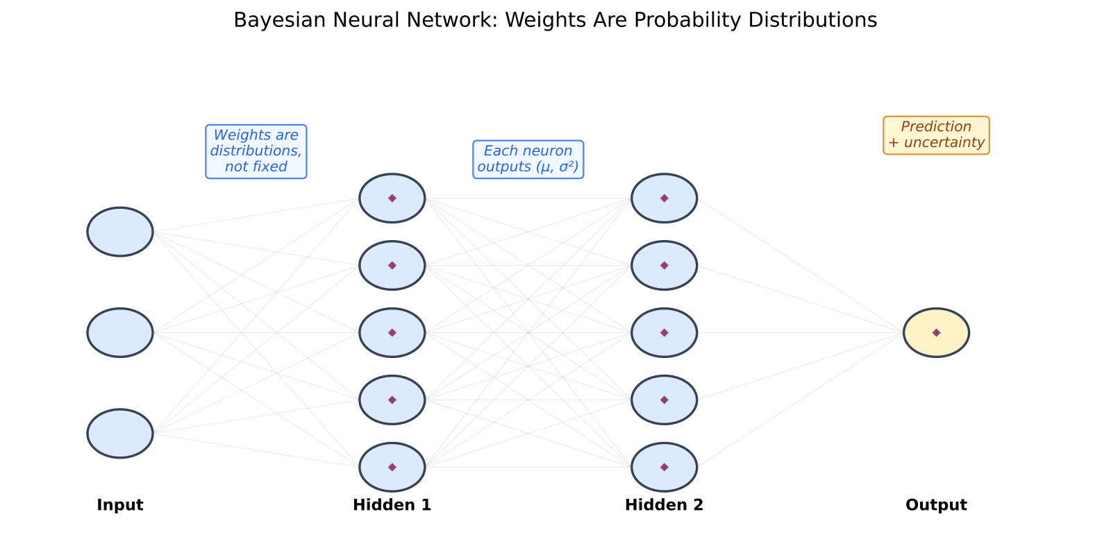
A Bayesian Neural Network (BNN) treats every weight as a probability distribution instead of a fixed number. Where a standard network stores one value per weight, a BNN stores two: a mean (the best guess) and a standard deviation (how sure it is about that guess). During training, the network learns not just “what value should this weight be” but “how much should this weight be allowed to vary.” When you feed an input through the network, each weight samples from its distribution, producing a slightly different output each time. The spread of those outputs is your uncertainty estimate.

Take a single weight with mean 0.30 and standard deviation 0.05. Feed the same input x = 2 through the network five times. Each time, the weight draws a different sample from its distribution, and you get a different output:

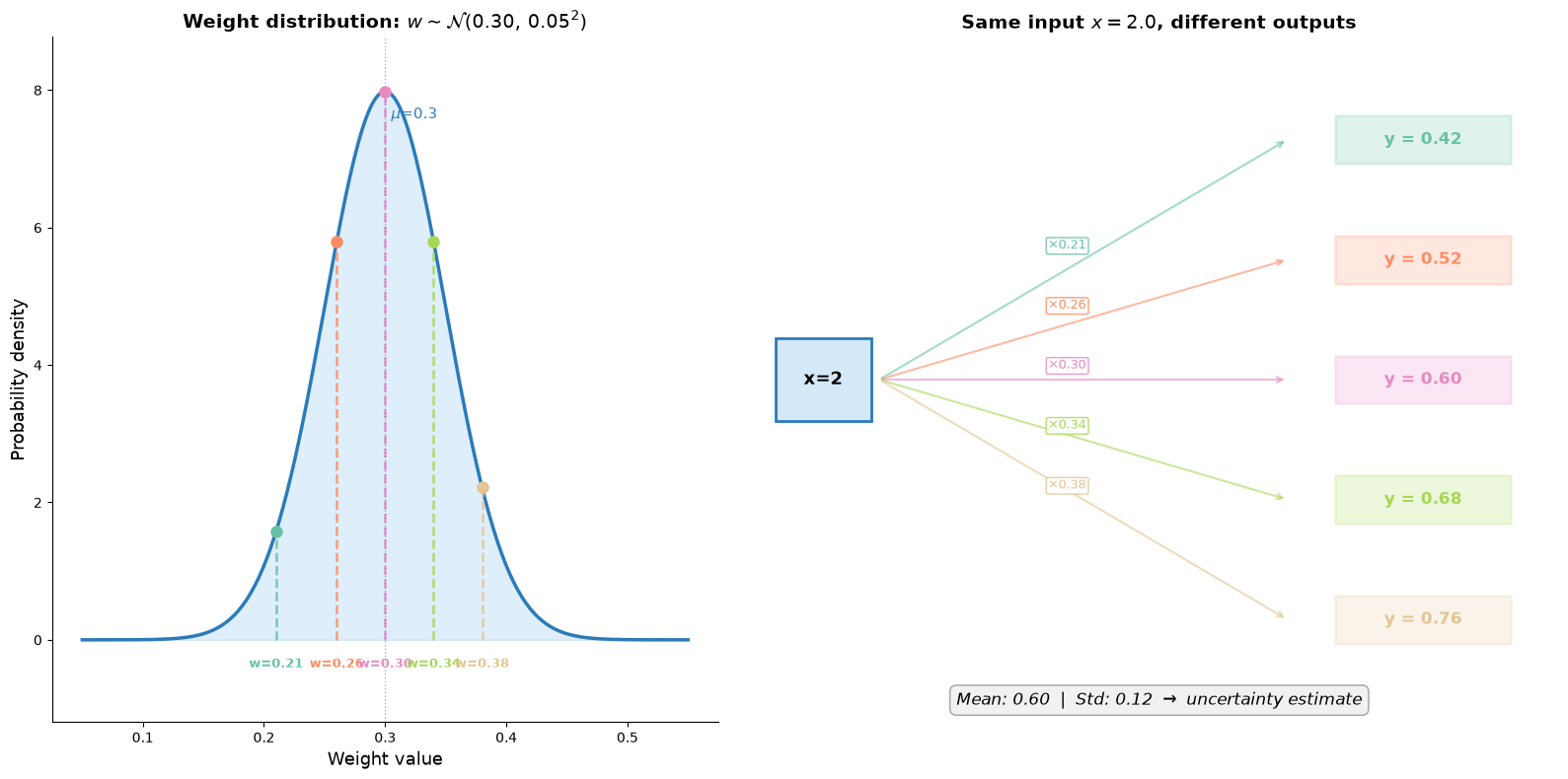
The spread of those outputs (std = 0.12 in this example) is your uncertainty estimate. A weight with a tight distribution (small std) always gives nearly the same output, so the network is confident about what that weight should be. A weight with a wide distribution produces a large spread, meaning the network is uncertain. Multiply this across thousands of weights and you get a principled measure of how much the network’s prediction could vary.

Why uncertainty matters

For most machine learning applications (image classification, recommendation, language modeling) you do not need uncertainty. You need the best guess, and if the model is wrong, it is wrong.

Trading is different. The cost of being wrong scales with how much you bet. If your volatility model says 0.35 and the true value is 0.30, you lose a little. If it says 0.35 and the true value is 0.90, you lose a lot. A model that says “0.35 but I am not sure” lets you size your position accordingly. Bet small when uncertain, bet big when confident. A model that just says “0.35” gives you no way to distinguish the two situations.

I use this for predicting crypto prices. When the model’s epistemic uncertainty is high, the prediction is unreliable and you should not act on it. Without uncertainty, you have no way to know when to sit out.

Dropout and ensembles are the two common alternatives for uncertainty estimation. Dropout (Gal and Ghahramani, 2016) is cheap but gives a narrow view. It only captures uncertainty from randomly zeroing activations, not from the full weight posterior. Ensembles (Lakshminarayanan et al., 2017) are better calibrated but require training and storing N separate models. BNNs give you a full posterior approximation from a single model, at the cost of doubling the parameter count (mean + std per weight) and needing a more careful training procedure.

How BNN training works

The standard neural network loss is just “make predictions match targets.” The BNN loss has two terms:

Data likelihood: How well do the current weight samples explain the training data? This is the same MSE or cross-entropy you would use in a standard network, except you sample the weights before each forward pass.

KL divergence: How far have the learned weight distributions drifted from the prior? The prior is your initial belief about what the weights should look like, typically a zero-mean Gaussian with some standard deviation. The KL term penalizes the network for becoming too confident (collapsing weight distributions to point estimates) or too weird (drifting far from zero). It is the Bayesian regularizer: it prevents overfitting by keeping the posterior close to the prior.

The total loss is data_loss + beta * KL, where beta controls the tradeoff. Small beta means “trust the data more, let the weights do what they want.” Large beta means “stay close to the prior, be conservative.” This is the Evidence Lower Bound (ELBO) from variational inference, with a tunable temperature.

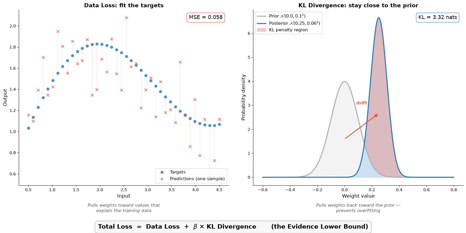
The left panel shows the data loss: predictions (red crosses) should land near the targets (blue dots). The residual lines show where they miss. The right panel shows the KL divergence: the learned posterior (blue, shifted and narrower) has drifted from the prior (gray, centered at zero). The pink shaded region is the penalty, where the KL term pushes the posterior back toward the prior, preventing the network from becoming overconfident. These two forces are in tension, and beta sets the balance.

Training uses the reparameterization trick (Kingma and Welling, 2013; Blundell et al., 2015): instead of sampling weights directly (which is not differentiable), you compute weight = mu + sigma * epsilon where epsilon is standard normal noise. This lets gradients flow through the sampling operation, so you can train with standard backpropagation. Each forward pass uses a different noise draw, so the network sees its own uncertainty during training.

The inference cost problem

After training, you have a distribution over weights. To get a prediction with uncertainty, the standard approach is Monte Carlo sampling: run the network 50 times with different weight samples, collect 50 different outputs, compute mean and standard deviation. The mean is your prediction; the standard deviation is your uncertainty.

This works, but 50 forward passes where you need one is a 50x overhead. For low-latency applications, that is a dealbreaker. You either give up uncertainty or give up speed.

Unless you can compute the uncertainty analytically in a single pass. That is possible, but only with the right activation function.

The activation function

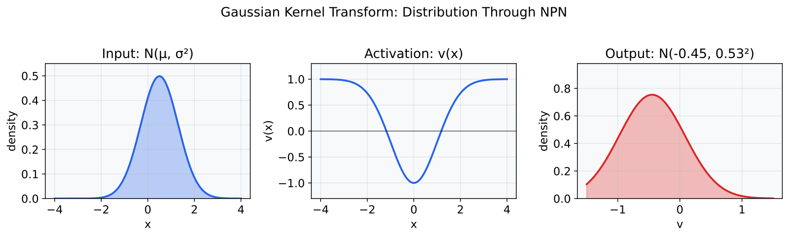
The NPN activation comes from Wang et al. 2016 (“Natural-Parameter Networks”, NeurIPS), who proved that for any exponential-family distribution, the activation v(x) = r - qexp(-tauu_i(x)) yields closed-form moments. I use the Gaussian case where u_i(x) = x^2:

v(x) = 1 - 2 * exp(-x^2/2)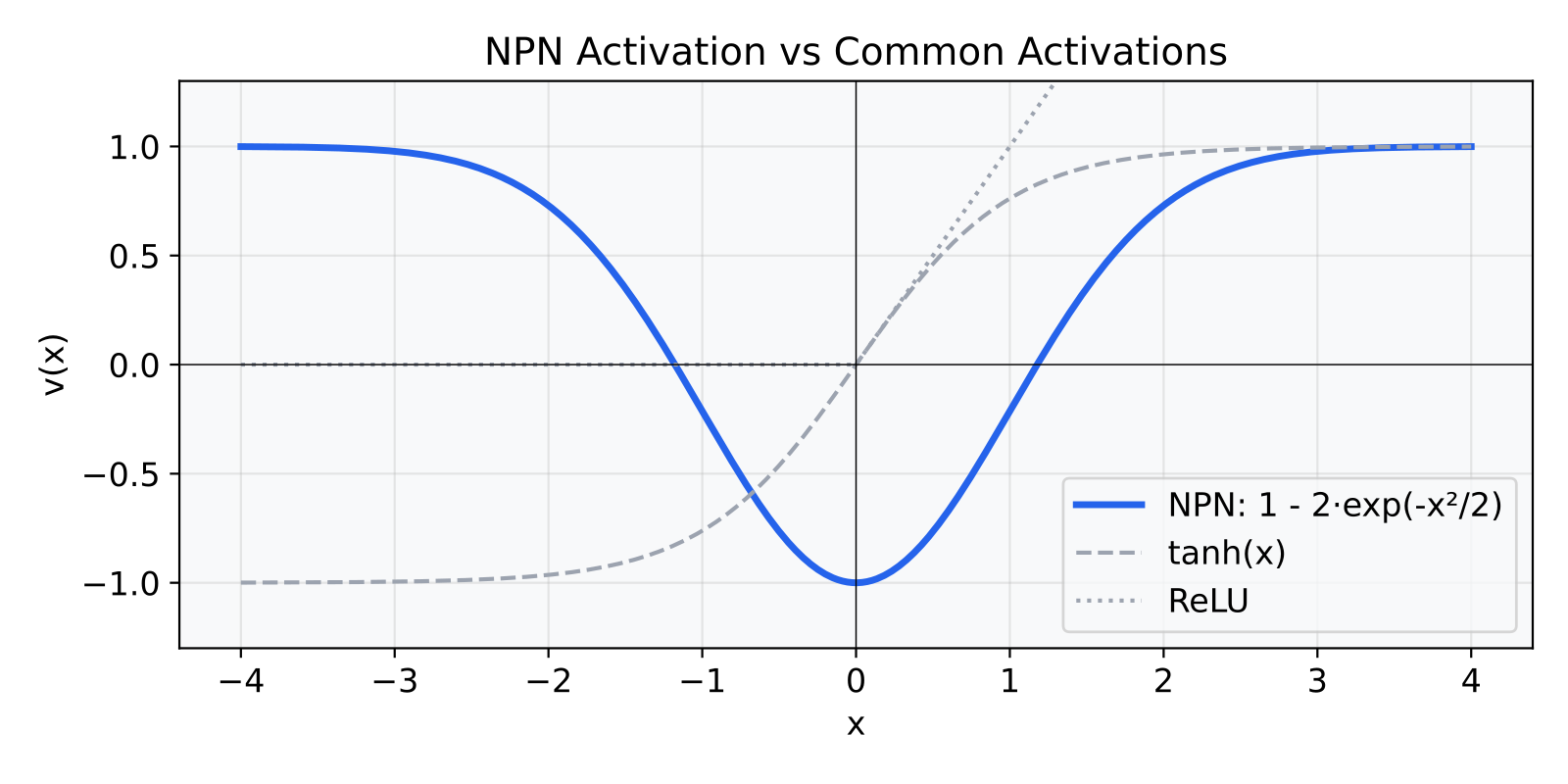

It has a deep valley at x=0 where the output is -1, then smooth walls rising on both sides, flattening out at +1 for large |x|. It is symmetric: v(x) = v(-x). Looks like a smoothed absolute-value function, or a Gaussian bump flipped upside down.

Why this function specifically? Because of what happens when you push a distribution through it instead of a single number.

The Gaussian kernel transform

In a BNN, the input to each neuron is not a fixed number. It is a Gaussian distribution N(mu, sigma^2). I need E[v(X)] and Var[v(X)] to propagate uncertainty through the network. For most activations (ReLU, SiLU, GELU), these expectations have no closed-form solution. You are stuck with sampling or crude approximations.

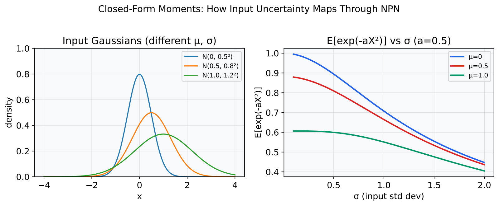
Normally, pushing a Gaussian through a nonlinear function gives you something that is no longer Gaussian, and the closed-form properties are gone. But exp(-ax^2) is special. The exponential-quadratic form meshes perfectly with the Gaussian’s own exponential-quadratic density, and the integral collapses:

E[exp(-aX^2)] = 1/sqrt(1 + 2asigma^2) exp(-amu^2 / (1 + 2asigma^2))

Just exp and sqrt, no special functions or numerical integration. A standard result from Gaussian integration: complete the square in the combined exponent, then use the normalization of the Gaussian PDF. The technique goes back to Weierstrass’s 1885 proof of the approximation theorem, where he used Gaussian convolution to smooth continuous functions.

Since NPN is a constant minus a Gaussian bump, both E[v(X)] and Var[v(X)] fall out in closed form.

The Fourier analogy

This clicked for me when I realized it is the same pattern as the Fourier transform, with a different basis:

	Fourier World	Gaussian World
Basis functions	sin(omegax), cos(omegax)	exp(-ax^2)
Transform	F(omega) = integral f(x) e^{-iomegax} dx	W(mu,sigma^2) = integral f(x) N(x; mu,sigma^2) dx
Convolution	Convolution theorem	Moment propagation
“Nice” functions	Bandlimited	Exponential-quadratic family
Closure	e^{iomegax} is eigenfunction of Fourier	Gaussian family closed under convolution

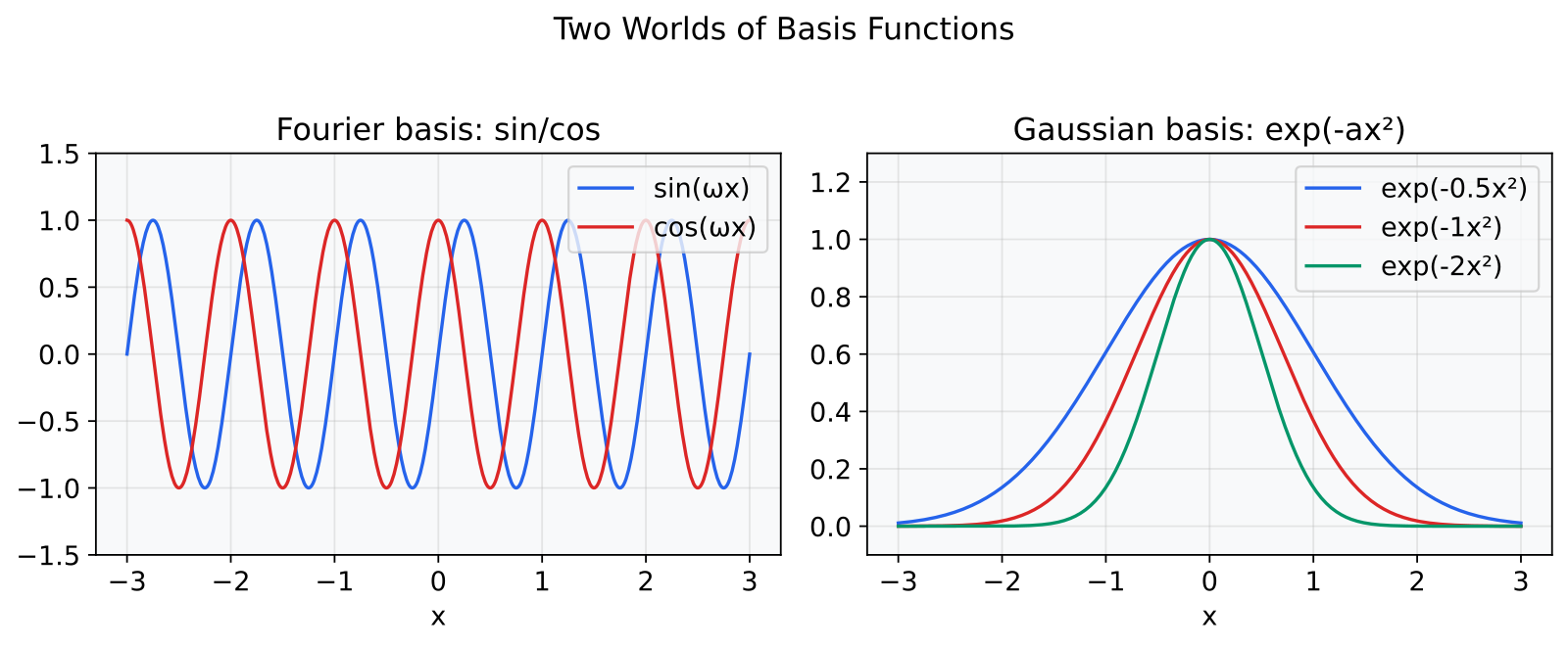
The Fourier transform decomposes signals into sine waves. The Gaussian transform decomposes functions into their behavior under uncertainty. A Gaussian convolved with a Gaussian is still a Gaussian, and that closure property is why NPN moments stay in closed form. Functions outside this family (sigmoid, ReLU) break the pattern and need approximation.

Probabilistic forward pass

Gast and Roth (CVPR 2018) formalized the idea of propagating (mean, variance) pairs through a network with closed-form activations as the “Probabilistic Forward Pass” (PFP), using Assumed Density Filtering. My implementation is a stripped-down version optimized for low-latency inference.

With NPN, I propagate (mean, variance) through the network. The first two layers are exact under the mean-field assumption:

1. Linear layer y = Wx + b: The output variance has three terms, from uncertainty in the weights, uncertainty in the inputs, and their interaction: Var(y) = E[x^2]Var(w) + E[w]^2Var(x) + Var(w)*Var(x). (This follows from expanding Var(WX) = E[(WX)^2] - E[WX]^2 and separating independent terms.) It is exact when input features are uncorrelated, which holds at the first layer.
2. NPN activation: Exact. The Gaussian kernel transform gives E[v(X)] and Var[v(X)] with exp and sqrt.
3. Output squashing: I use exp(-h^2/2) to keep the output bounded. Still in the exponential-quadratic family, still exact under mean-field. The non-monotonic shape (symmetric bell curve) works here because volatility is a magnitude: both large positive and large negative returns produce similar volatility responses. For tasks requiring monotonic output scaling (like classification), erf(x) would be the right choice within the same family.

The remaining approximation is diagonal covariance: after a linear layer, output features are correlated, but I only track the variance of each feature independently (no cross-feature covariance). This is an O(d) vs O(d^2) tradeoff. At random initialization it introduces about one order of magnitude error in variance estimates, but it tightens after training as weight variances shrink toward their posterior values. Weight standard deviations in the hidden layers cluster around the prior (0.08 to 0.12 post-training), while the output layer collapses to near-zero (~0.004). The network is confident about how to map its last hidden representation to a volatility estimate but uncertain about the internal features. The diagonal assumption means it underestimates uncertainty when features are strongly correlated.

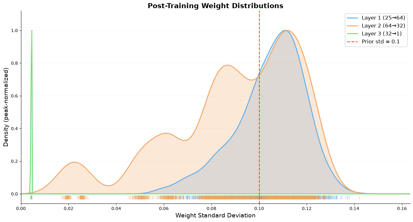
Each curve shows how uncertain the weights in one layer are after training. The tick marks along the x-axis are individual weights. Layers 1 and 2 (the hidden layers, with 1,600 and 2,048 weights respectively) spread broadly around the prior std of 0.1. The network has not squeezed out their uncertainty. Layer 3 (the output layer, 32 weights) has collapsed to a tight spike near 0.004. The network is very confident about its final mapping from hidden features to volatility. This is the right behavior: preserve uncertainty in the internal representations while committing to a specific output transform.

The family of closed-form activations

NPN is not the only option. Any function built from exp(-ax^2) terms has exact Gaussian moments:

• NPN v(x) = r - qexp(-taux^2/2). My workhorse. Bounded, smooth, exact.
• Cosine v(x) = cos(omegax). E[cos(omegaX)] = cos(omegamu)exp(-omega^2*sigma^2/2). Bounded gradients everywhere, connects to Random Fourier Features (Rahimi and Recht 2007).
• Asymmetric NPN v(x) = r - qexp(-tau(x-c)^2/2). Replace mu with (mu-c) in all formulas. Could capture the leverage effect (volatility responds asymmetrically to positive vs negative returns).
• Learnable tau. Same formula, tau per neuron. Each neuron picks its own sensitivity width.
• Mixture of Gaussians v(x) = sum a_k exp(-b_k x^2). Universal approximator within the exponential-quadratic family. O(K^2) cost for the cross terms.
• NPN + Linear v(x) = alphax + (1-alpha)(r - qexp(-taux^2/2)). Gradient highway like a residual connection. Breaks boundedness though, which is dangerous for variance propagation.

I am currently running NPN. Cosine is the most interesting alternative to try next. Its gradients do not saturate exponentially like NPN’s do for |x| > 3.

What went wrong

This was not a clean path from idea to working code.

Sigmoid was not in the family. My output layer originally used sigmoid to bound the prediction. Sigmoid has no exact Gaussian moments. I had to use a heuristic approximation with 10-30% error on the variance estimate. I eventually replaced it with exp(-h^2/2), which is in the exponential-quadratic family. Zero approximation error.

Float32 cancellation. The variance formula computes E[G^2] - E[G]^2. When the input variance is tiny (< 10^-7), both terms are nearly identical, and the difference goes negative due to floating-point cancellation. Analytically it is always >= 0 (that is the definition of variance), but float32 does not care about your proofs. Fixed with .clamp(min=0). The PFP path runs under no_grad, so gradient behavior at the boundary is irrelevant.

Zero gradient at the origin. The derivative of exp(-h^2/2) is h*exp(-h^2/2), which is zero at h=0. Unlike sigmoid (which has maximum gradient at zero), the NPN output squashing has a dead zone right where the network initializes. I fixed this by biasing the last layer’s initialization away from zero.

Diagonal covariance. This is the approximation I live with. After a linear layer, features are correlated through the shared weight matrix. I only track the diagonal of the covariance matrix. The error is architecture-dependent and tightens after training. For my 3-layer BNN with 96 hidden neurons (64 + 32), it is good enough.

Performance

Tested on BTC 1-minute klines, [64, 32] hidden layers, 7,557 parameters. Three seeds, 100K rows each, MPS (Apple GPU) inference.

NPN vs SiLU training

Metric	NPN	SiLU
Best val QLIKE	0.929	0.931
Time/epoch	1.40s	1.66s
Total (50 epochs)	74.5s	88.1s

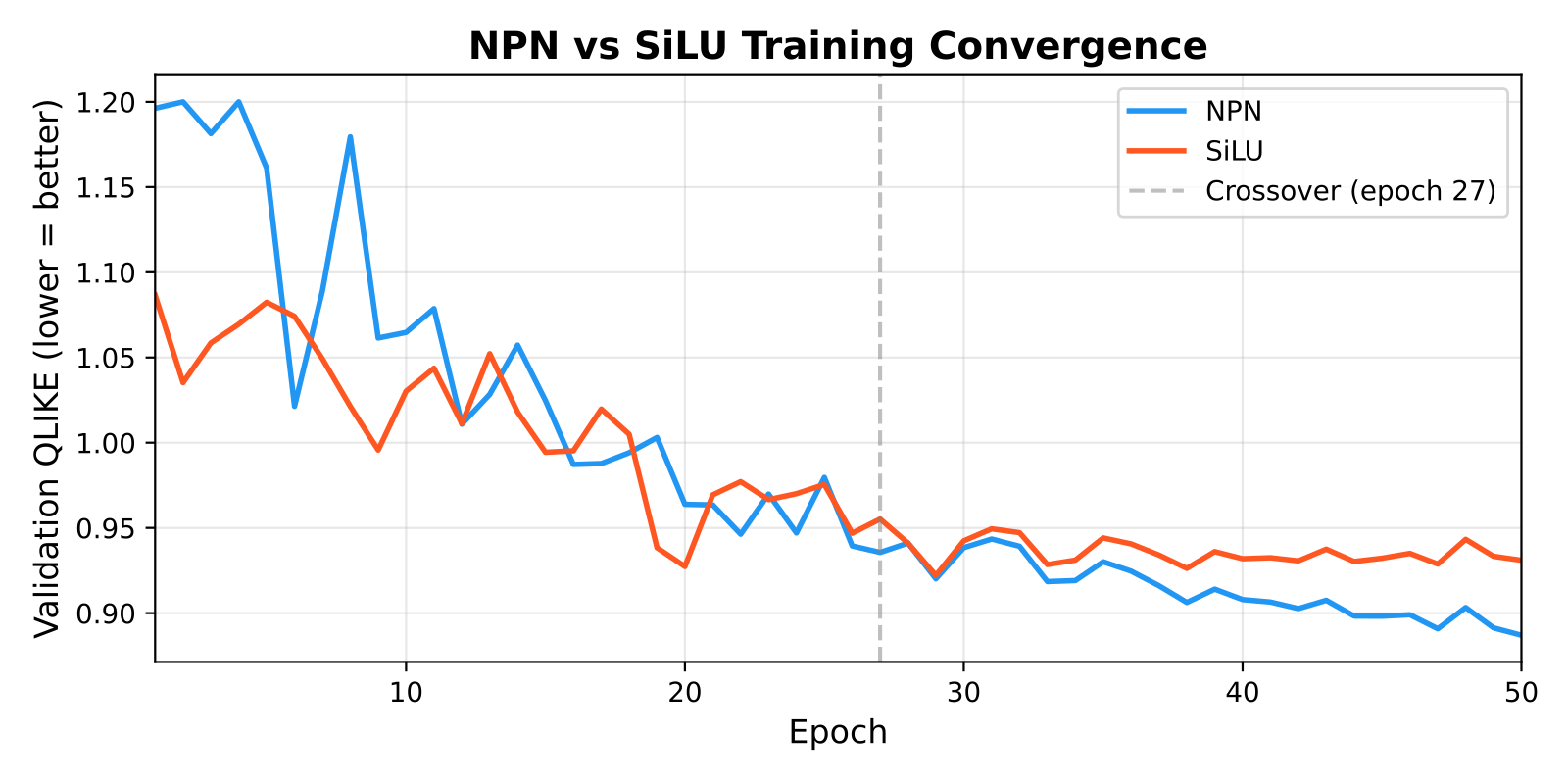
NPN starts slower (epoch 10: 3.33 vs 1.35, because the Gaussian bump sits in its dead zone near h=0 early on), but overtakes SiLU around epoch 27. Trains 16% faster per epoch due to fewer memory-bound operations in the activation path.

Inference speed: Laplace vs Monte Carlo

Method	Time	QLIKE	Correlation	Speedup vs MC(20)
Deterministic	0.049s	0.882	0.399	—
Laplace (analytical)	0.077s	0.882	0.399	18x
MC(20)	1.418s	0.918	0.398	baseline
MC(50)	3.654s	0.916	0.401	—

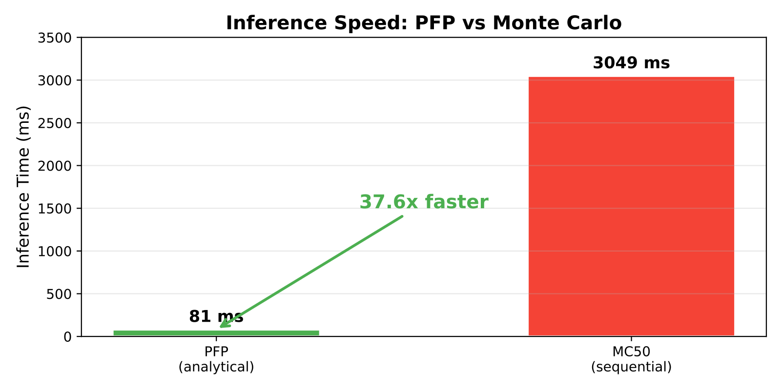
Three-seed average. Laplace preserves exact point predictions (same QLIKE and correlation as deterministic) while providing epistemic uncertainty in a single forward pass. MC(20) and MC(50) add sampling noise that slightly worsens QLIKE. Epistemic uncertainty correlation between Laplace and MC(20) is ~0.43. They capture overlapping but not identical signals.

The MC baseline runs sequential forward passes on CPU. A vectorized GPU implementation would close the gap to 3-5x, but for low-latency CPU inference, the 18x speedup is the realistic number.

I also found a neat optimization: fusing q/sqrt(d) exp(a) into a single exp(log(q) - 0.5log(d) + a) call. This eliminates both sqrt operations from the moment computation and gave me an 18x speedup on the _npn_moments function itself.

The deeper connection

Neal showed in 1996 that Bayesian neural networks converge to Gaussian Processes in the infinite-width limit. My NPN activation is exp(-x^2/2), which is related to the RBF kernel. The connection is not that my BNN is a GP with an RBF kernel (the limiting NNGP kernel of a BNN is computed via recursive inner-product expectations and is more complex than the activation itself). By choosing an activation in the exponential-quadratic family, I make mean-field variational inference analytically tractable: each forward pass propagates (mean, variance) pairs exactly under the diagonal covariance assumption, giving me a fast approximation to the posterior predictive without Monte Carlo sampling.

What’s next

• Cosine activation experiment: cos(omega*x) has better gradient properties than NPN for deep networks and preserves variance through deep stacks. Worth a training comparison.
• Hybrid covariance: Track the full 32×32 covariance matrix at the last hidden layer only. Cheap (1024 extra ops) and eliminates the diagonal approximation where it matters most.
• Deploy to production: Replace the existing volatility model with BNN+PFP for live inference.

Does any of this improve real-world performance? I do not know yet. The uncertainty signal should help avoid acting on unreliable predictions. That matters more than beating a linear baseline on a point-estimate metric, but I will not know for sure until it runs live.