TL;DR: Copy & paste the linked code to have working Neural Network as a starting point for your application
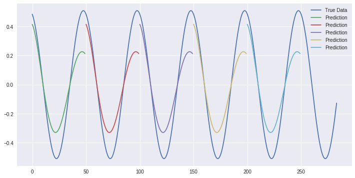
50 consecutive prediction steps on a sine wave. Source: mine
Introduction
I tried several times to get started with Deep Learning. But pretty much all the tutorials were outdated and it was just a lot of work with no result in the end.
This time I invested my time into learning a sine wave. And it actually works! I’ve published the Jupyter Notebook on Colaboratory which you can just copy and get started within 5 minutes.
How it works
This is based on my previous article Deep learning made easy with Colaboratory. You don’t have to install any software. The code is stolen from several github repositories.
The steps
Divide the task into steps. Finish each step, check if it has been successful, pat yourself on the back and take a break.
Step 0: generate data
You need time series data. Try a sine wave before you switch over to bitcoins and stocks. A sine wave has all kinds of nice properties like
- easy
- you know there is a repetitive structure inside which you could learn
- scaled between -1 and +1
- no trend (bitcoin has an upwards trend -> LSTM predicts prices will always rise)
I’ve realized that you should always visualize your data. Otherwise you will spend hours learning a 404 html page interpreted as a *.csv file. This is what a sine wave looks like:
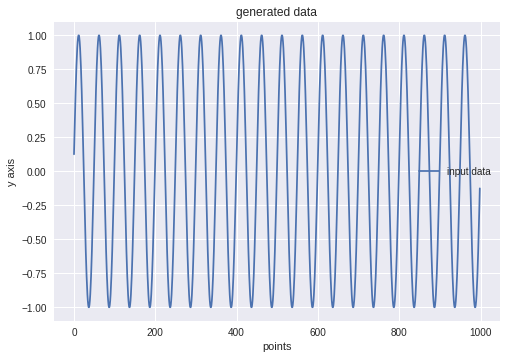
A sine wave. Source: Babylon, ca. 2000 BC
Step 1: Load data
Neural Networks are general function approximators. We are even using LSTMs which have a memory. Now we have to define our input and output space. These words sound like it would get complicated. But it won’t because I don’t know how to type the letters.
We take 50 points from the sine wave. And we predict the next step.
Neural Networks need a lot of training data. That’s why we cut the sine wave into 50 points long parts and take the next point as our desired output. We have 1000 discrete sine wave points which leads to 949 training examples.
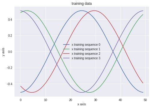
random training samples from the sine wave. Source: mine
Step 2: Build Model
This is where the magic is. I don’t really know how this code works. And likewise, you don’t have to.
I can tell you that this is called a LSTM neural network. LSTM stands for Long-Short-Term-Memory. That’s a Neuron which is really good for time series because it can remember previous input over varying time distances. It’s a neural network because we have 2 connected layers and each layer has a bunch of those LSTMs. All together, this is a structure in which you can imprint knowledge by learning and, during execution, this thing can also remember a tiny bit of the previous input.
def build_model(layers):
    model = Sequential()

    model.add(LSTM(
    input_shape=(layers[1], layers[0]),
    units=layers[1],
    return_sequences=True))
    model.add(Dropout(0.2))

    model.add(LSTM(
    layers[2],
    return_sequences=False))
    model.add(Dropout(0.2))

    model.add(Dense(
    units=layers[3]))
    model.add(Activation("linear"))

    start = time.time()
    model.compile(loss="mse", optimizer="adam")
    print("> Compilation Time : ", time.time() - start)
    return model
Step 3: Train the model
You feed your examples to the previously built model. This can take a lot of time and there are some magic numbers you have to set:
- epochs: defines how many times you want to to through all your data
- batch size: defines how much you want to load at once into the GPU memory
Afterwards you can extract how good the model performed from the history.
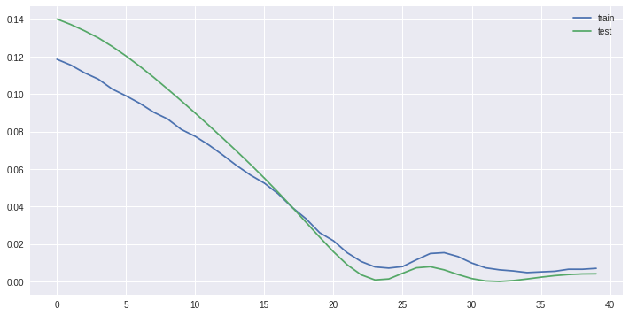
mean squared error vs epoch. source: mine
What’s nice about this is that the test data is “unknown” to the Neural Network. That is, it is not learnt. That’s your opportunity to see whether the network is overfitting. If it does, the error for the test data should rise.
Step 4: Plot the predictions
Remember the used input and output space: The output is just 1 step! But to make money we have to look into the future of bitcoin! We don’t want to predict one step, we want to predict the charts for the next weeks and invest our borrowed money.
Also, one step is too easy: You could just copy the previous value and you wouldn’t be that far off.
The code I stole makes a point by point prediction or dead reckoning. That is, the prediction is re-used as a new input value. That’s done 50 times. Here is my result:
50 consecutive prediction steps on a sine wave. Source: mine
Yay! We start at random points and predict 50 points. You can see that it almost matches the sine wave.
Next steps
But it’s not perfect. The way it is right now we would be leaving a lot of bitcoins on the table. We need better predictions for a bigger yacht. Or a second yacht and a helicopter.
That’s where you come in: Can you make the model better? Can you make it predict better? Just play around with it. That’s also how you would proceed if this wasn’t a toy problem. Just repeat the steps:
- is the data wrong? Could we improve the data by removing trends, outliers etc? (The answer is no. This is a sine wave)
- Can we do something better when loading the data? E.g. also load the volume, use the day of the week, use the previous day’s average price, use another timescale.
- the model. We are using 50 input neurons and 15 deep neurons. Using a bigger model means more capabilities means we improve performance? WTF is adam?
- learning. Can we learn more often? Less? Look at the loss function chart.
- your personal point of view: Are your assumptions about the problem and solution correct?
Conclusion
I had a lot of fun doing this and I hope you’ll have too. There is a lot of room for improvements, so just play around with it: Jupyter Notebook on Colaboratory